2 Background
Distress not yourself if you cannot at first understand the deeper mysteries of Spaceland. By degrees they will dawn upon you.
– Edwin A. Abbott, Flatland: A Romance of Many Dimensions, 1884
This chapter provides a succinct introduction to various topics discussed in the experimental chapters of this dissertation. Rather than a comprehensive review of relevant literature, it aims to provide key background about the research presented in this manuscript.
In particular, Section 2.1 and Section 2.4 discuss the basic functioning of neural networks-based language models and machine translation (MT) systems, and introduce the machine translation task representing the core focus of this work. Section 2.2 and Section 2.3 provide an introduction to methods for attributing inputs and conditioning generation in language models, corresponding to the topics discussed in Part I and Part II. Finally, Section 2.5 and Section 2.6 dive deeper in the translation domain, providing an overview of how MT models are employed in the translation industry by human post-editors, and discussing techniques for automatically evaluating machine translation quality. These notions provide a valuable background to Part III, which focuses on the impact of interpretability insights on human translation workflows.
Beyond this background section, each experimental chapter briefly summarizes relevant literature to contextualize the research questions and findings.
2.1 From Neural Networks to Neural Language Models
Neural networks are computational models which integrate principles from statistical learning theory (Vapnik, 1995), consisting of interconnected nodes (neurons) organized in layers, where each connection has an associated weight. Formally, a neural network is a function \(\mathbf{f}: \mathcal{X} \to \mathcal{Y}\) that maps inputs \(\mathbf{x} \in \mathcal{X}\) to outputs \(\mathbf{y} \in \mathcal{Y}\), where \(\mathcal{X}\) and \(\mathcal{Y}\) are the input and output feature spaces, respectively. The function \(\mathbf{f}\) is parameterized by weights \(\mathbf{\theta} \in \Theta\), which are typically learned from data through the training process described in Section 2.1.1. Individual neurons are functions parametrized by weights \(\mathbf{w} \in \mathbb{R}^d\) and biases \(b \in \mathbb{R}\), which are combined to produce an output \(\sigma(\mathbf{w}^T\mathbf{x} + b)\), where \(\sigma\) is a non-linear activation function. Thanks to non-linearities, sequences of neurons can learn to represent complex relations from input vector \(\mathbf{x}\).1
2.1.1 Supervised Learning for Neural Networks
In the supervised learning paradigm, given a training dataset \(\mathcal{D}\) containing paired instances:
\[\mathcal{D} = \{(\mathbf{x}_1, y_1), \ldots, (\mathbf{x}_N, y_N)\} \in (\mathcal{X} \times \mathcal{Y})^n \tag{2.1}\]
where \(\mathbf{x}_i\) is a vector of input features and \(\mathbf{y}_i\) is the expected output, a neural network is trained to learn a functional mapping \(\mathbf{f}\) from inputs \(\mathbf{x}\) to labels \(\mathbf{y}\) by minimizing the average value of a loss function \(\ell: \mathcal{Y} \times \mathcal{Y} \to \mathcal{R}\), such that \(\ell(\mathbf{f}(\mathbf{x}), \mathbf{y})\) quantifies the gap between predicted outcomes \(\tilde{y}\) and ground truth \(y\) over examples in \(\mathcal{D}\). The function \(\mathbf{f}\) is parameterized by weights \(\mathbf{\theta} \in \Theta\), which are optimized during training so as to minimize the loss function. Such optimization is typically performed using some variant of stochastic gradient descent (SGD), in which iterative steps \(1, \dots, t \dots, T\) are taken to update \(\mathbf{\theta}\) in the direction of the negative gradient of the loss function with respect to the weights:
\[\mathbf{\theta}_{t+1} \leftarrow \mathbf{\theta}_t - \eta \;\nabla_{\mathbf{\theta}} \,\ell(\mathbf{f}(\mathbf{x}_j; \mathbf{\theta}_t), \mathbf{y}_j) \tag{2.2}\]
where \(\eta\) is a chosen learning rate, and \(\mathbf{x}_j\) and \(\mathbf{y}_j\) are a subset of randomly sampled input-output pairs from the training set \(\mathcal{D}\), typically referred to as mini-batch. This iterative refinement of model parameters is repeated until convergence, i.e. until the model performance on a left-out validation set does not improve significantly, allowing for a robust convergence to a local minimum of the loss function, even for non-convex problems and high-dimensional parameter spaces.
We commonly refer to the inference process going from input \(\mathbf{x}\) to output \(\mathbf{y}\) as forward pass, and to the process of computing gradients and updating model parameters as backward pass.
2.1.2 Transformer Neural Networks
Transformers (Vaswani et al., 2017) are a class of neural networks that have become the de-facto standard for most natural language processing tasks, constituting the core neural network architecture employed throughout this thesis’ experiments. In essence, a transformer consists of a sequence of identical macro-layers, dubbed blocks, progressively contextualizing a sequence of input features \(\mathbf{Z} \in \mathbb{R}^{S \times d}\), where \(S\) is the sequence length and \(d\) is the size of each feature vector. Figure 2.1 illustrates the structure of a single transformer module, constituting the core of decoder-only language models such as GPT-3 (Brown et al., 2020) presented later in Section 2.1.3. Notably, the transformer architecture is characterized by its ability to process input sequences in parallel, as opposed to recurrent models (Rumelhart and McClelland, 1987; Hochreiter and Schmidhuber, 1997), making it highly efficient for training on large datasets.
We now describe the main components of a transformer block in order of execution during the forward pass, using \(\mathbf{z}_i \in \mathbb{R}^d\) to denote the input representations at each component for sequence element \(i\). This will be useful for explaining steering intervention and vocabulary projection methods used in Chapter 7 and Chapter 10, respectively.
Layer normalization (LN). The layer normalization operation, also known as LayerNorm (Ba et al., 2016), is a common approach for stabilizing the training process of deep neural networks. In practice, layer normalization applies the transformation:
\[\text{LN}(\mathbf{z}_i) = \frac{\mathbf{z}_i - \mu(\mathbf{z}_i)}{\sigma(\mathbf{z}_i)} \odot \gamma + \beta \tag{2.3}\]
where \(\mu, \sigma\) are the mean and the standard deviation of \(\mathbf{z}\), and \(\gamma, \beta\) are learnable scale and bias parameters for the normalization. This operation helps to mitigate issues related to internal covariate shift, improving convergence during training. Recently, LayerNorm has been substituted with RMSNorm (Zhang and Sennrich, 2019), which removes the mean centering step and scales the input using the root mean square (RMS) statistic.
Multi-head self-attention (MHSA). The self-attention mechanism is the core component of the transformer architecture, allowing the model to contextualize its representations at each layer by combining information across the input sequence. While the original formulation of multi-head self-attention by Vaswani et al. (2017) involves a concatenation of attention head outputs before the final output projection, we follow here the more recent formulation by Kobayashi et al. (2021) and Elhage et al. (2021), which reformulates the attention output computation using the sum of individual attention heads, emphasizing the linear reading and writing operations within the attention computation.
Concretely, the self-attention module is composed by a series of \(H\) attention heads \(\text{Attn}_1, \ldots, \text{Attn}_H\), each computing the following weighted sum:
\[\text{Attn}_h(\mathbf{z}_i) = \sum_{j} \alpha^h_{ij} \mathbf{z}_j \mathbf{W}_V \mathbf{W}_O \tag{2.4}\]
Intuitively, the sharding of the attention mechanism into separate computations can be beneficial when processing the complex relations within different elements of the input sequence, for example, the lexical, syntactic and semantic dimensions of words in a text. The learnable weight matrices \(\mathbf{W}_V \in \mathbb{R}^{d \times d_h}\) and \(\mathbf{W}_O \in \mathbb{R}^{d_h \times d}\), where \(d_h\) represents the dimension of each head, can be combined into the so-called output-value (OV) circuit as \({\mathbf{W}_V \mathbf{W}_O = \mathbf{W}_{OV} \in \mathbb{R}^{d \times d}}\). For every key \(j\) given the current query position \(i < S\), the corresponding attention weight \(\alpha^h_{i}\) is computed as:
\[\alpha^h_{i} = \text{softmax}(\frac{\mathbf{z}_i \mathbf{W}_Q (\mathbf{W}_K \mathbf{Z})^T}{\sqrt{d_h}}) \tag{2.5}\]
Once again, the learnable weight matrices \(\mathbf{W}_Q \in \mathbb{R}^{d \times d_h}\) and \(\mathbf{W}_K \in \mathbb{R}^{d \times d_h}\) can be combined as the query-key (QK) circuit \({\mathbf{W}_Q \mathbf{W}_K^T = \mathbf{W}_{QK} \in \mathbb{R}^{d \times d}}\). This decomposition enables a view of QK and OV circuits as the units responsible for reading from (QK) and writing to (OV) the residual stream. Finally, the attention block output is the sum of individual attention heads: \[\text{Attn}(\mathbf{z}_i) = \sum_{h=1}^{H} \text{Attn}_h(\mathbf{z}_i) \tag{2.6}\]
Residual connection. The introduction of residual connections (He et al., 2016) in the transformer architecture allows the model to learn identity mappings more easily, facilitating the training of deeper networks and avoiding the vanishing gradient problem (Hochreiter, 1998). A residual connection is commonly applied to the output of the self-attention module, resulting in:
\[\text{ResAttn}(\mathbf{z}_i) = \text{Attn}\big(\text{LN}(\mathbf{z}_i)\big) + \mathbf{z}_i \tag{2.7}\]
Feedforward network (FFN). The feedforward network (FFN) in the transformer block is composed of two learnable weight matrices2: \(\mathbf{W}_{\text{in}} \in \mathbb{R}^{d \times d_{\text{ffn}}}\) and \(\mathbf{W}_{\text{out}} \in \mathbb{R}^{d_{\text{ffn}} \times d}\). \(\mathbf{W}_{\text{in}}\) reads from the residual stream state \(\mathbf{z}\), and its result is passed through an element-wise non-linear activation function \(\sigma\), producing a set of neuron activations. These get transformed by \(\mathbf{W}_{\text{out}}\) to produce the output \(\text{FFN}(\mathbf{z})\):
\[\text{FFN}(\mathbf{z}_i) = \sigma(\mathbf{z}_i \mathbf{W}_{\text{in}}) \mathbf{W}_{\text{out}} \tag{2.8}\]
The FFN operation was compared to a retrieval step from a key-value memory (Geva et al., 2021), with keys stored in columns of \(\mathbf{W}_{\text{in}}\) acting as pattern detectors over the input sequence, and values in rows of \(\mathbf{W}_{\text{out}}\) being upweighted by respective neuron activation. The overall block structure from Figure 2.1 can then be summarized as:
\[\text{Block}(\mathbf{z}_i) = \text{FFN}\Big(\text{LN}\big(\text{ResAttn}(\mathbf{z}_i)\big)\Big) + \text{ResAttn}(\mathbf{z}_i) \tag{2.9}\]
We will henceforth use \(\mathbf{z}_i^l\) to denote the output of the \(l\)-th block for the \(i\)-th element of the input sequence for transformer models.
2.1.3 Transformer Language Models
A language model is a probabilistic model that can assign probabilities to sequences of tokens. Formally, given an input sequence \(\mathbf{X} = \langle t_1, \dots, t_S \rangle\) of \(S\) tokens, which in the case of natural language are typically words or subword units (Sennrich et al., 2016) from a vocabulary \(\mathcal{V}\), a language model \(f\) computes the probability of the sequence as the product of token-level conditional probabilities:
\[P(\mathbf{X}) = P(t_1, \dots, t_S) = \prod_{i=1}^{S} P(t_i|t_1, \dots, t_{i-1}) \tag{2.10}\]
Language models operating under such formulation are typically referred to as auto-regressive or causal language models (CLMs, or simply LMs), to differentiate them from masked language models (MLMs) trained to fill the blanks in a sequence (Devlin et al., 2019). While MLMs were the main object of analysis of early interpretability research on transformer models (Tenney et al., 2019; Clark et al., 2019; Rogers et al., 2020), this dissertation focuses solely on CLMs, which after the advent of ChatGPT3 in 2022 became the dominant paradigm in the NLP and interpretability community. CLMs are typically decoder-only models, following the structure introduced in Section 2.1.2, or encoder-decoder models, such as the MT systems later discussed in Section 2.4.
Importantly, LMs can be used for generating text by iteratively sampling from the probability distribution over the next token \(t_{i}\) given the previous tokens \(t_1, \dots, t_{i-1}\), e.g. using the greedy decoding sampling method:
\[t_i^* = \underset{t \in \mathcal{V}}{\arg\,\max}\;P(\,\cdot\,|t_1, \ldots, t_{i-1}) \tag{2.11}\]
This sampling process can be repeated autoregressively, i.e. by adding the selected token \(t_i^*\) to the input sequence, until a special end-of-sequence token is generated, or until a maximum sequence length is reached.
We now turn to the additional components required to convert the generic transformer model presented in the previous section into a language model able to process and generate sequences of tokens. Figure 2.2 shows a stylized view of a transformer LM.
Embedding layer. The first component of a transformer language model is the embedding layer, which maps input tokens to continuous vector representations, known as embeddings. Word embeddings such as Word2Vec (Mikolov et al., 2013) and GloVe (Pennington et al., 2014) revolutionized the field of natural language processing by exploiting distributional semantics, i.e. the fact that words which frequently appear in similar contexts should have similar meaning (Harris, 1954), to learn word representations end-to-end using gradient descent. In transformers, the token embedding matrix \(\mathbf{E} \in \mathbb{R}^{|\mathcal{V}| \times d}\), where \(d\) is the size of the embedding vectors, and \(|\mathcal{V}|\) is the vocabulary size, is learned jointly with the rest of model parameters during training. The embedding layer maps each token \(t_i\) in the input sequence to its corresponding vector \(\mathbf{z}_i = \mathbf{E}[t_i]\). The resulting sequence of embeddings \(\mathbf{Z} \in \mathbb{R}^{S \times d}\) corresponds to the input to the first transformer block. It is important to note that representations produced by \(\mathbf{E}\) are not contextualized, i.e. the same token \(t_i\) will always be mapped to the same vector \(\mathbf{z}_i\), regardless of its meaning in the given sequence. For example, the word ring will always be mapped to the same vector, regardless of whether it is used as a noun or a verb. The transformer blocks are used to contextualize these representations, i.e. produce different vectors for the same token depending on the remainder of the sequence.
Positional encodings. While the sequential nature of language is an important factor in how we produce and process linguistic information, transformer models do not explicitly account for ordering across elements of the input sequence. For this reason, positional encodings injecting information about the position of each token in the sequence are commonly used in transformer-based language models. The most basic positional encoding is a fixed sinusoidal encoding (Vaswani et al., 2017), which is added directly to the input embeddings. Recent models, however, employ rotary position embeddings, allowing for the encoding of both absolute and relative positions between tokens, and allowing the model to generalize to longer contexts beyond those seen during training (Su et al., 2024).
Causal self-attention. The self-attention mechanism in transformer language models is causal, meaning that the attention weights for each token \(t_i\) are computed only over the tokens preceding it in the sequence, i.e. \(t_1, \ldots, t_{i-1}\). This ensures that the model can only attend to past tokens when predicting the next token, preserving the auto-regressive nature of the model. The causal self-attention mechanism is implemented by masking out future tokens in the attention computation, ensuring that \(\alpha^h\) is computed only for \(j \leq i\) in Equation 2.4, and that only representations \(Z_{\leq i}\) are used to compute the key vector in Equation 2.5.
Prediction head. The prediction head of a transformer language models consists of a so-called unembedding matrix \(\mathbf{W}_{U} \in \mathbb{R}^{d \times |\mathcal{V}|}\) mirroring the initial embedding operation, sometimes accompanied by a bias. The last residual stream state \(\mathbf{z}_S^L\), where \(L\) is the number of transformer blocks and \(S\) is the sequence length, gets transformed by this linear map converting the representation into a next-token distribution of logits, which is turned into a probability distribution via the softmax function:
\[P(\,\cdot\,|t_1, \ldots, t_{i-1}) = \text{softmax}(\mathbf{z}_i^L \mathbf{W}_{U}) \tag{2.12}\]
In light of the residual stream view presented in Section 2.1.2, showing that different model components read from and write to the residual stream, it is natural to believe that the predictions derived by applying the unembedding matrix to the final residual stream state \(\mathbf{z}_S^L\) are the product of an iterative refinement across model components (Jastrzebski et al., 2018). The logit lens method (nostalgebraist, 2020), which we study for error detection in Chapter 10, exploits this intuition to analyze how the model refines the prediction throughout the forward pass, by projecting intermediate residual stream states \(\mathbf{z}_S^l\), with \(l < L\), to the vocabulary space using \(\mathbf{W}_{U}\).
Language model pre-training. Modern language models such as those employed in this thesis are typically pre-trained on large web corpora spanning billions or trillions of tokens using the next-token prediction objective, i.e. minimizing the cross-entropy loss between the next-token distribution predicted by the model and the next observed token. This frames the language model training problem as an instance of supervised learning, which we presented in Section 2.1.1. Formally, given a minibatch \(D_t\) of corpus \(\mathcal{D}\) composed by sequences of tokens \(\mathbf{X_k} = \langle t_1, \ldots, t_{S_k} \rangle\), the loss for a single training step is computed as:
\[\mathcal{L}_{\text{step}} = -\frac{1}{|D_t|} \sum_{\mathbf{X_k} \in D_t} \sum_{i=1}^{S_k} \log P(t_i|t_1, \ldots, t_{i-1}) \tag{2.13}\]
Concretely, this corresponds to maximizing the likelihood of the observed tokens given the context provided by the preceding tokens, while minimizing the likelihood of all other incorrect tokens.
Language model post-training. After pre-training, language models can be used for generating text given some context, but mostly lack the ability to perform specific tasks without being provided explicit examples, or respond to queries as conversational agents. For this reasons, all language models used for our experiments underwent additional supervised fine-tuning (SFT, also known as instruction tuning), allowing them to learn input-output mappings for realistic user queries beyond natural text occurrences in the pre-training corpus (Howard and Ruder, 2018; Sanh et al., 2022). The fine-tuning process still involves the same \(\mathcal{L}_{\text{step}}\) loss function over a smaller, curated set of demonstrations. Some of the models we study—such as the Gemma 2 models from Chapter 7 or the Zephyr model from Chapter 5 —underwent an additional reinforcement learning from human feedback (RLHF) step, in which the model is fine-tuned to maximize the likelihood of human preferences over pairs of model generations, using a reward model trained on human preferences. This process is typically performed using Proximal Policy Optimization [PPO;Schulman et al. (2017)] or similar reinforcement learning algorithms. Unless otherwise specified, we use the term language model to refer to transformer language models that were first pre-trained and then fine-tuned, representing the main focus of this thesis.
2.2 Explaining Predictions with Input Attribution
Contrary to linear models, where learned coefficients directly correspond to the influence of their respective features towards predictions, neural networks’ outcomes cannot be directly interpreted due to the presence of multiple nonlinearities across layers, rendering the attribution of model prediction to individual input features non-trivial. Input attribution methods, also known as feature attribution, were introduced to address this issue by providing a principled way to assign importance scores to input features, clarifying the rationales behind model decisions (Zeiler et al., 2011).
Formally, for a model \(\mathbf{f} \in \mathcal{F}: \mathcal{X} \to \mathcal{Y}\), given an input \(\mathbf{x} \in \mathcal{X}\), we can define the attribution method \(\gamma\) as a functional:
\[\gamma: \mathcal{X} \times \mathcal{F} \to \mathbb{R}^{|\mathcal{X}|}\]
so that \(\mathbf{a}_{\mathbf{f}(\mathbf{x})} = \gamma(\mathbf{x}, \mathbf{f})\) is a vector of attribution scores quantifying the influence of each element of \(\mathbf{x}\) on the model predictive distribution \(\mathbf{f}(\mathbf{x})\), with higher scores representing greater importance (Fel, 2024). It is worth noting that attribution methods can rely on one or more specific outcomes \(\mathbf{y} \in \mathcal{Y}\) from the predictive distribution \(\mathbf{f}(\mathbf{x})\), such as perturbation-based approaches (Covert et al., 2021), or simply rely on the flow of information within the model to identify important input elements (Abnar and Zuidema, 2020). We call the former methods target-dependent, and we discuss them further in Chapter 4.
2.2.1 Attribution Method Categories
We now briefly summarize common families of input attribution methods, which are employed throughout the first part of this thesis. An in-depth overview of input attribution techniques for natural language processing can be found in Madsen et al. (2022).
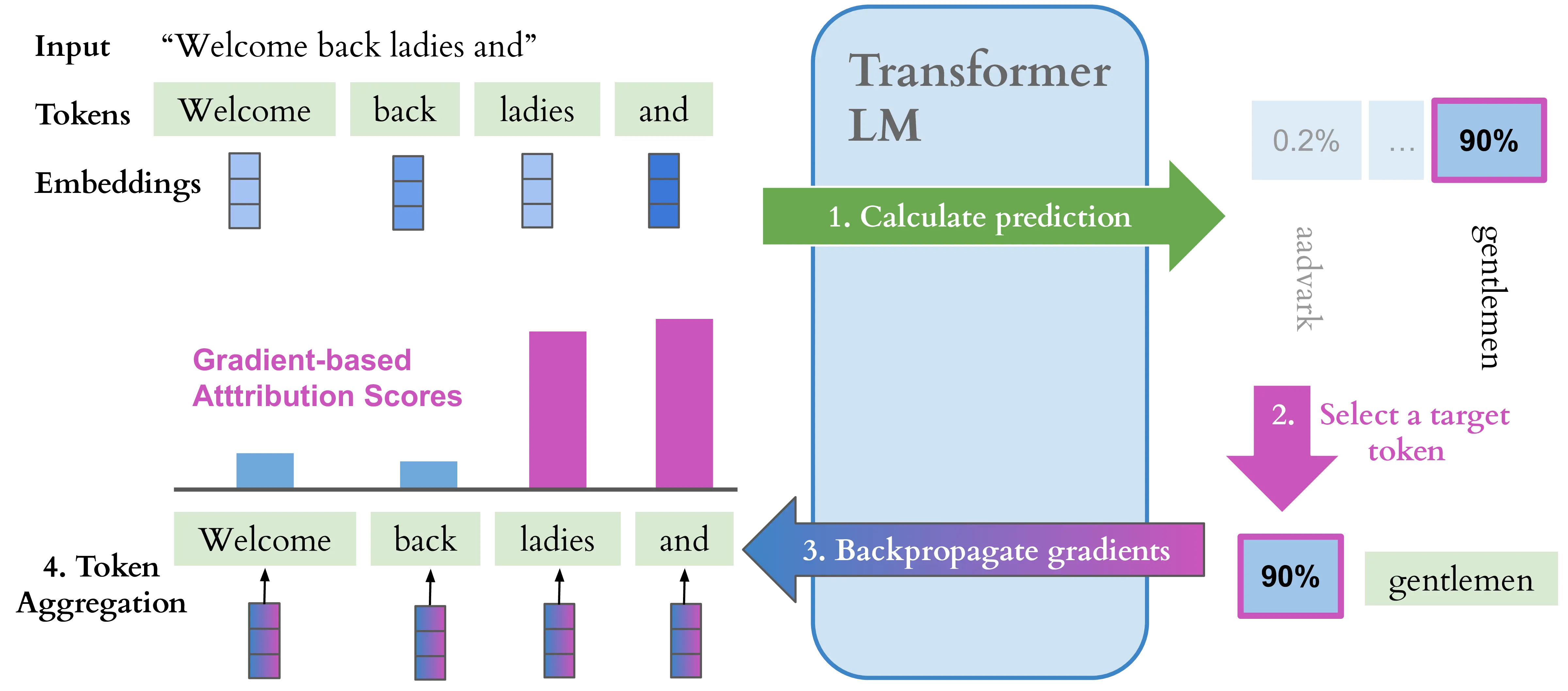
Gradient-based attribution For neural network models like transformer LMs, gradients are a natural source of input saliency which can be exploited for attribution purposes (Simonyan et al., 2014; Li et al., 2016). A simple gradient-based attribution corresponds to a first-order Taylor expansion of the model at a point \(\mathbf{x}\), expressed as \(\nabla \mathbf{f}(\mathbf{x}) \cdot \mathbf{x} + \mathbf{b}\). The resulting gradient \(\nabla_\mathbf{x}^c {\mathbf{f}}\) captures intuitively the sensitivity of the model prediction \(c\) to each element in the input. In the case of transformer LMs, \(\nabla_\mathbf{x}^{t^*} {\mathbf{f}} \in \mathbb{R}^{S \times d}\), i.e. every dimension of the input embedding is associated with a attribution score, and the logit of the top predicted token \(t^*\) is used as differentiation target for gradient computation.4 These scores are generally aggregated at a token level to obtain a more intuitive overview of the influence of individual tokens. This is commonly done by taking the \(L^p\) norm of the gradient vector:
\[\text{Grad}_{\,\mathbf{f}(\mathbf{x}) \leftarrow t^*} = \|\nabla_{\mathbf{x}}^{t^*} \mathbf{f}\|_p \in \mathbb{R}^{S} \tag{2.14}\]
Figure 2.3 shows an example of gradient attribution on a language model. By taking the dot product between the gradient vector and the input embedding \({\nabla_{\mathbf{x}}^{t^*} \mathbf{f}\cdot \mathbf{x}}\), known as the gradient \(\times\) input method, this sensitivity information can be converted to an importance estimate. More elaborate gradient-based attribution methods employ perturbations of the input embedding (Sundararajan et al., 2017; Smilkov et al., 2017) or ad-hoc gradient propagation rules (Bach, 2015; Achtibat et al., 2024) to filter noisy gradient information.
Gradient-based attribution methods are heavily used in the investigations of Chapter 3, Chapter 4 and Chapter 5, representing the majority of methods supported by the Inseq toolkit and the most effective approaches for contextual cues imputation in the PECoRe framework. Notably, gradient attribution can be exploited in a similar way to identify the importance of intermediate states \(\mathbf{z}\) in the model, as opposed to input representations \(\mathbf{x}\), i.e. using \(\nabla_{\mathbf{z}}^{t^*} \mathbf{f}\). The CAT method proposed in Chapter 3 case study adopts this attribution-based approach to locate factual knowledge across LM layers.
Perturbation-based attribution Another popular family of approaches estimates input importance by adding noise or ablating input elements and measuring the resulting impact on model predictions. For instance, the input token \(w_j\) at position \(j\) can be removed, and the resulting probability difference \(p(t^*|t_{<i}) - p(t_{\setminus w_j}^*|t_{<i})\), where \(t^*\) is the predicted token for current sequence position \(i\) and \(j < i\), can be used as an estimate for its importance. If the logit or probability given to \(w\) does not change, we conclude that the \(i\)-th token has no influence. A multitude of perturbation-based attribution methods exist in the literature, such as those based on local surrogate models such as LIME (Ribeiro et al., 2016), or those derived from game theory like SHAP (Lundberg and Lee, 2017). Notably, some architecture-specific methods such as Value Zeroing (Mohebbi et al., 2023) have been proposed to mitigate the disruptive impact of perturbations on model behaviors. A comprehensive framework unifying various perturbation-based approaches is presented by Covert et al. (2021).
Context mixing for attribution Model internals such as the attention weights \(\alpha\) presented in Section 2.1.2 were initially proposed as possible explanations for model behavior (Bahdanau et al., 2015), but were found unfaithful in reflecting the actual predictive behavior of language models (Jain and Wallace, 2019; Bastings and Filippova, 2020). This is because, contrary to other approaches, they only accounted for the importance of specific model components, rather than a more general notion of saliency across the full model. However, recent methods have proposed more refined estimates of token contributions exploiting internals to quantify the information flow within LMs. Some of these alternatives include the use of the norm of value-weighted vectors and output-value-weighted vectors (Kobayashi et al., 2020; Kobayashi et al., 2021), or the use of vectors’ distances to estimate token contributions (Ferrando et al., 2022). These methods result in a set of attribution scores \(\mathbf{a}_{\mathbf{f}(\mathbf{x})} \in \mathbb{R}^{S \times L}\), marking the contribution of position-specific representation across all layers \(1, \ldots, L\) of the model. These per-layer attributions reflecting context mixing patterns are often aggregated using techniques such as rollout (Abnar and Zuidema, 2020), resulting in one score per input token participating in the attention operation. Such context mixing approaches have shown competitive faithfulness compared to best gradient and perturbation-based methods, despite employing only a single forward pass to estimate contributions.
Contrastive input attribution An important limitation of input attribution methods for interpreting language models is that attributed output tokens belong to a large vocabulary space, often having semantically equivalent tokens competing for probability mass in next-word prediction (Holtzman et al., 2021). In this context, attribution scores are likely to misrepresent several overlapping factors such as grammatical correctness and semantic appropriateness driving the model prediction. Recent work addresses this issue by proposing a contrastive formulation of such methods, producing counterfactual explanations for why the model predicts token \(t^*\) instead of an alternative token \(t^\sim\). Yin and Neubig (2022) extend the vanilla gradient method of Equation 2.14 to the contrastive setting as:
\[\text{ContGrad}_{\,\mathbf{f}(\mathbf{x}) \leftarrow t^*, t^\sim} = \nabla_{\mathbf{x}}^{t^* - t^\sim} \mathbf{f} \tag{2.15}\]
We employ this formulation in the PECoRe framework in Chapter 4 and its extension of Chapter 5 to identify salient context cues for generated tokens that were highly influenced by context.
2.2.2 Evaluating and Using Attribution Methods
Plausibility and Faithfulness The evaluation of input attribution methods can be operationalized in terms of various desiderata. Plausibility, also referred to as “human-interpretability” (Lage et al., 2019), is a measure of “how convincing the interpretation is to humans” (Jacovi and Goldberg, 2020), i.e. how well the salient tokens identified by an attribution method are in agreement with those selected by human annotators. It is important to note that plausibility does not imply faithfulness, i.e. how accurately the rationale reflects the true reasoning process of the model (Wiegreffe and Pinter, 2019), since a good explanation of model behavior might not align with human intuition. Consider the following sentence from the BLiMP corpus (Warstadt et al., 2020).
\(\mathbf{x}\) = A report about the Impressionists has/\(*\)have won the competition.
For the sentence to be grammatically correct, the verb to have must be correctly inflected as has to agree with the preceding noun report. Hence, to evaluate the plausibility of a language model for this example, the model is provided with the prefix \(\mathbf{x}'\) =“A report about the Impressionists”. Then, attribution scores are computed for every input token towards the prediction of has as the next token. Finally, we verify whether these scores identify the token report as the most important to predict has. We note that the selection of the pair report-has in the canonical procedure described above is entirely based on grammatical correctness, and other potential pairs not matching these constraints are not considered (e.g. the usage of report to predict writing instead of has as a likely continuation). This common procedure might also cause reasonable behaviors to be labeled as implausible. For example, the indefinite article A might be identified as the most important token to predict has since it is forcibly followed by a singular noun and can co-occur with has more frequently than report in the model’s training data. These limitations in the standard hypothesis-driven approach to plausibility evaluation motivate our proposal for PECoRe as a data-driven alternative in Chapter 4.
Limitations of input attribution methods While input attribution methods are commonly used to debug failure cases and identify biases in models’ predictions (McCoy et al., 2019), popular approaches were shown to be insensitive to variations in the model and data generating process (Adebayo et al., 2018; Sixt et al., 2020), to disagree with each others’ predictions (Atanasova et al., 2020; Crabbé and Schaar, 2023; Krishna et al., 2024) and to show limited capacity in detecting unseen spurious correlations (Adebayo et al., 2020; Adebayo et al., 2022). Importantly, popular methods were found provably unreliable at predicting counterfactual model behavior in realistic settings (Bilodeau et al., 2024). Apart from theoretical limitations, perturbation-based approaches also suffer from out-of-distribution predictions induced by unrealistic noised or ablated inputs, and from high computational cost of targeted ablations for granular input elements.
Tools for input attribution The captum library (Kokhlikyan et al., 2020) is part of the Pytorch ecosystem providing access to several gradient and perturbation-based input attribution methods for any Pytorch-based model, with the recent addition of utilities for simplifying attribution analyses of generative LMs (Miglani et al., 2023). Several captum-based tools provide convenient APIs for input attribution of transformer-based models, notably Transformers Interpret (Pierse, 2021), ferret (Attanasio et al., 2023) and Ecco (Alammar, 2021), which are mainly centered around language classification tasks. SHAP (Lundberg and Lee, 2017) is a popular toolkit mainly centered on perturbation-based input attribution methods and model-agnostic explanations for various data modalities. The saliency library5 provides framework-agnostic implementations for mainly gradient-based input attribution methods, while LIT (Tenney et al., 2020) is a framework-agnostic tool providing a convenient set of utilities and an intuitive interface for interpretability studies spanning input attribution, concept-based explanations and counterfactual behavior evaluation. It notably includes a visual tool for debugging complex LLM prompts (Tenney et al., 2024). More recent low-level interpretability tools such as nnsight (Fiotto-Kaufman et al., 2025) also support attribution, without explicitly providing abstractions to facilitate its usage. inseq, which we introduce in Chapter 3 as part of this thesis’ contributions, is one of the most popular tools for input attribution of generative LMs, supporting advanced approaches for contrastive context attribution (Sarti et al., 2024) and context mixing evaluation.
2.3 Conditioning Language Model Generations
This section describes the two main families of approaches for conditioning the behavior of language models during text generation. First, we present methods for modifying the input context by providing relevant information retrieved from external sources, or demonstrations of desired behavior, which we use in Chapter 5, Chapter 6, and 7. Then, we discuss approaches for modifying the model’s internal representations to achieve targeted interventions in the generation process, which we compare to prompting methods in Chapter 7.
2.3.1 Controlling Input Context
Large language models have become widely popular due to their ability to adjust their predictions in light of few examples or relevant information provided in an input context (prompt), without requiring additional training (Brown et al., 2020). Prompting LLMs to exploit their in-context learning skills has become pervasive in the NLP community, with much effort devoted to designing effective prompts for various tasks (Dong et al., 2024).
Few-shot prompting is an effective approach to adapt LLMs to new tasks by providing a few demonstrations of the desired behavior in the input context. For example, to perform a translation, a few source language examples can be provided in the prompt with their respective target language translations, and the model is expected to translate new source entries used as queries (Figure 2.4, left). Zero-shot prompting is a more challenging task, where the model is expected to perform well on a new task without any demonstrations, relying solely on its pre-trained knowledge. While effective, several studies highlighted the brittleness of prompting to unexpected factors such as the order of provided examples (Lu et al., 2022). In this thesis, we use few-shot prompting in our attribute-controlled translation experiments of Chapter 6 and our literary translation experiments of Chapter 7.
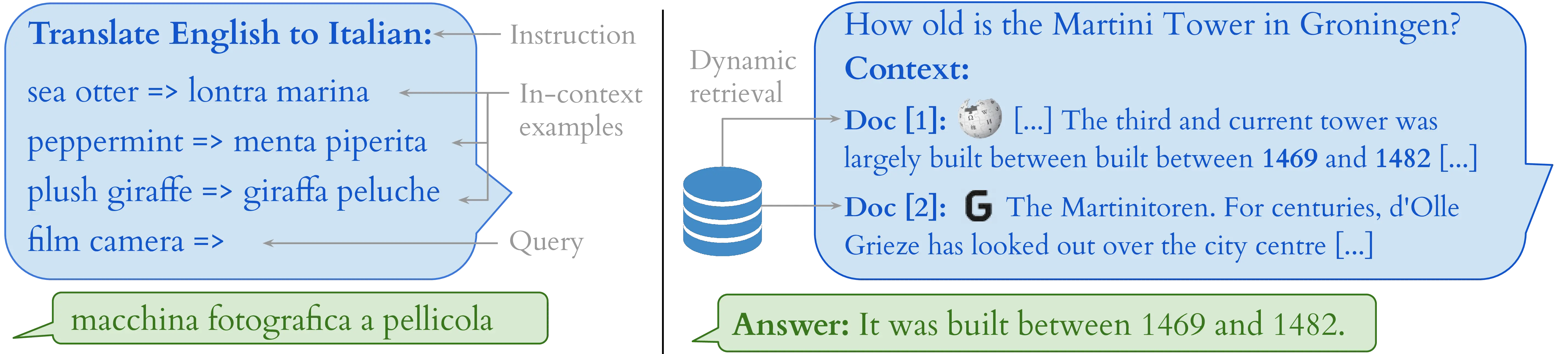
Retrieval-augmented generation (RAG) is a different approach for conditioning generation where the model is provided with relevant context paragraphs retrieved on-the-fly from an external dataset, such as Wikipedia or a domain-specific corpus. This context is then used to inform the model’s predictions, allowing it to generate more accurate and relevant responses without relying solely on its potentially faulty pre-training knowledge (Figure 2.4, right). RAG has been shown to be effective in improving the factual accuracy of model outputs and reducing hallucinations (Lewis et al., 2020; Petroni et al., 2020). However, it is not directly obvious which retrieved paragraphs are motivating the model’s predictions, a challenge we address via input attribution in Chapter 5. Chapter 6 also employs a similarity retrieval component to control the examples selected for few-shot prompting, showing that example selection leads to better performances in machine translation with LLMs.
2.3.2 Controlling Model Representations
Techniques for conditioning model behavior by modifying the model’s internal representations are commonly referred to as steering methods, and often exploit the linear structure of model activations to achieve simple targeted interventions. Indeed, the linear representation hypothesis states that latent properties of interest—for example, the tone of a response—are encoded as linear subspaces of the representation space in language model activation (Park et al., 2023). Such property was already observed in early work on word embeddings (Mikolov et al., 2013), where the direction of the vector between two words was shown to encode their semantic relationship, e.g. \(\mathbf{z}_{\text{king}} - \mathbf{z}_{\text{man}} + \mathbf{z}_{\text{woman}} \approx \mathbf{z}_{\text{queen}}\).
Recent work highlighted the effectiveness of linear interventions on language models representations using directions identified by a probing classifier, i.e. a model \(\mathbf{p}: \mathbb{R}^{d} \to \mathcal{C}\) trained to predict a specific property of interest \(c \in \mathcal{C}\) from the intermediate representation of a trained transformer LM (Köhn, 2015; Gupta et al., 2015; see Belinkov, 2022 for a review). For instance, adding negative multiples of the sentiment direction (\(\mathbf{c}_\text{sent}\)) to the residual stream, i.e. modifying the activation \(\mathbf{z}^l\) as \({\tilde{\mathbf{z}}^l \leftarrow \mathbf{z}^l - \alpha \mathbf{c}_\text{sent}}\), where here \(\alpha\) is a pre-selected steering coefficient controlling the intensity of the intervention, is sufficient to generate a text exhibiting the opposite sentiment label (Tigges et al., 2024). This simple procedure, known as activation addition, has become popular for conditioning desired attributes in model generations, including multiple properties at once (Scalena et al., 2024). Some of its variants omit probing classifiers and employ other unsupervised methods for computing feature directions, such as K-Means clustering of representations for examples showing a desired property (Zou et al., 2024), or mean difference between representations for positive and negative sets of demonstrations (Marks and Tegmark, 2024; Arditi et al., 2024).
Wu et al. (2024) describe a broader framework for representation steering, proposing the use of learnable interventions for conditioning generation at specific steps with variable intensity. Formally, an intervention \(I\) can be defined as a tuple composed by an intervention function \(\xi: \mathbb{R}^d \to \mathbb{R}^d\) with learnable parameters, a set of input positions \(P \subseteq \{1, \dots, S\}\) that the intervention is applied to and the layer \(l\) at which the intervention is applied. This framework, dubbed representation fine-tuning (ReFT), allows to learn interventions overriding \(\mathbf{z}^l\) as:
\[z^l_i = \begin{cases} \xi(\mathbf{z}^l_i), & \text{if}\; i \in P \\ \mathbf{z}^l_i, & \text{otherwise} \end{cases} \tag{2.16}\]
The intervention function can be learned by minimizing the normal cross-entropy loss with a next token prediction objective, optimizing only the parameters of the intervention function. Activation addition (ActAdd) can then be described as a special case in this broader framework, where the intervention function \(\xi\) is constant and applied at all generation steps. In the experiments of Chapter 7, we use ActAdd and ReFT as baselines for our proposed steering method.
The final steering approach we discuss in this section involves the use of sparse autoencoders[SAEs; Huben et al. (2024)] for conditioning model behavior. SAEs have become widely adopted for analyzing the representations learned by transformer LMs thanks to their ability to address polysemanticity, i.e. the entanglement of multiple concepts within learned model representations. Indeed, neurons in transformer LMs were observed to activate on diverse and semantically distinct contexts, with concepts being encoded in a distributed manner across multiple units (Smolensky, 1986; Olah, 2023). In light of this, and given the disparity between the relatively low-dimensional representations learned by transformer LMs and the vast array of abilities they acquire during training, latent concept representations were speculated to be encoded in superposition across various model units (Arora et al., 2018), i.e. that multiple neurons jointly encode the presence of a single concept (Figure 2.5, left). A concrete example of this phenomenon is given by Elhage et al. (2022), where superposition is observed in presence of a long tail of sparse concepts in the training dataset.
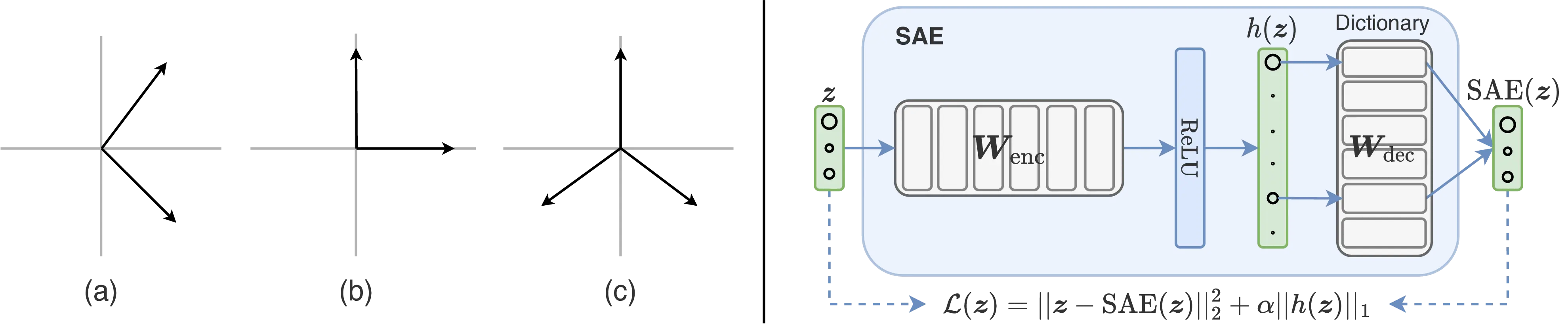
A possible strategy to disentangle concepts in superposition involves finding an overcomplete feature basis via dictionary learning (Olshausen and Field, 1997; Donoho and Elad, 2003). SAEs are simple autoencoder neural networks, i.e. models trained to reconstruct their input, that can be trained to reconstruct internal representations \(\mathbf{z} \in \mathbb{R}^{d}\) of a neural network exhibiting superposition. Their training objective encourages the model to learn a sparse coding of the input representation through an ad-hoc loss term, resulting in a sparse dictionary of learned concepts. Huben et al. (2024) and Bricken et al. (2023) propose training SAEs on transformer LM representations using the form:
\[ \begin{aligned} \text{SAE}(\mathbf{z}) &= h(\mathbf{z})\,\mathbf{W}_{\text{dec}} + \mathbf{b}_{\text{dec}} \\ \text{with}\; h(\mathbf{z}) &= \sigma\big((\mathbf{z} - \mathbf{b}_{\text{dec}})\mathbf{W}_{\text{enc}} + \mathbf{b}_{\text{enc}}\big) \\ \end{aligned} \tag{2.17}\]
using the loss function:
\[\mathcal{L}(\mathbf{z}) = \|\mathbf{z} - \text{SAE}(\mathbf{z})\|_2^2 + \alpha \|h(\mathbf{z})\|_1 \tag{2.18}\]
where \(\sigma\) is a non-linear activation function, \(\mathbf{W}_{\text{enc}}\) and \(\mathbf{W}_{\text{dec}}\) are the encoder and decoder learned weight matrices, respectively, and \(\alpha\) is a hyperparameter controlling the sparsity of the learned representation. The first term in Equation 2.18 is the reconstruction term, accounting for the quality of reconstruction, while the second term is the sparsity term, which promotes sparsity. The SAE architecture is illustrated in Figure 2.5 (right).
If \(h(\mathbf{z}) \in \mathbb{R}^{m}\) and \(m \gg d\), \(\mathbf{z}\) can be approximated as a sparse linear combination of the learned rows in the dictionary \({\mathbf{W}_{\text{dec}} \in \mathbb{R}^{m \times d}}\), ideally representing monosemantic concepts. Similarly to activation addition, these concepts can be used to steer model behavior by scaling them using a steering coefficient before reconstruction, resulting in a modified representation \(\tilde{\mathbf{z}}\). We use a similar approach in our SAE-based steering method we present in Chapter 7.
2.4 Machine Translation
Machine translation is a long-standing task in natural language processing, with the goal of automatically translating text from a source language to another target language. In this section, we provide a brief overview of the evolution of machine translation approaches, describe how transformer LM architectures are commonly used for machine translation, and how such models can handle multiple languages and contextual information.
The history of machine translation can be summarized in three main phases. Between the 1960s and the 1980s, the first successes of machine translation were attained by rule-based systems exploiting various techniques, ranging from direct translation using dictionaries with a set of reordering rules to ambitious methods aiming to exploit an interlingua to act as a bridge when mapping meaning across languages (Hutchins, 2001). As for most rule-based methods, however, these approaches were limited by the need of ad-hoc rules, which could hardly account for less frequent and challenging settings. From the 1990s onwards, the statistical paradigm took foot by exploiting large bilingual corpora made available by the birth of the World Wide Web to train statistical language models parametrized as tables of co-occurrence probabilities (Och et al., 1999), with popular approaches aiming to segment challenging sentences into simpler phrases for ease of translation via co-occurrences (Koehn et al., 2003) or syntactic analysis (Hadiwinoto, 2017). In 2013, the advent of word embeddings coincided with the first MT systems based on continuous language representations parametrized by neural networks (Kalchbrenner and Blunsom, 2013), marking the advent of the neural MT (NMT) paradigm that remains the current state-of-the-art for machine translation. While the architecture of NMT systems has barely changed since the introduction of the transformer, as for most NLP tasks the introduction of large pre-trained language models has led to general-purpose models able to handle various translation-related task via light tuning and ad-hoc prompting (Alves et al., 2024).
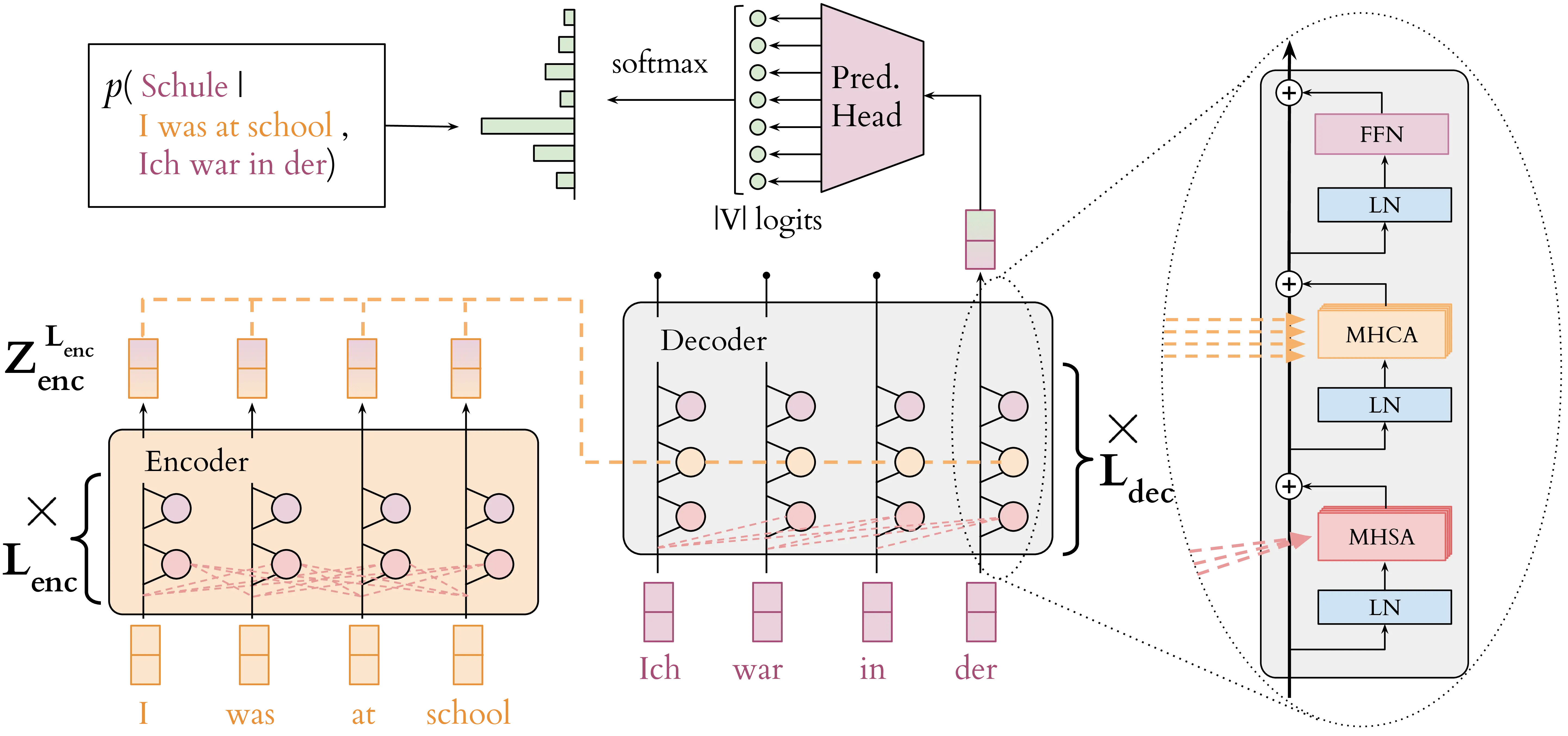
Provided that machine translation involves the generation of a sequence of translated target tokens, it is straightforward to see how such task can fit well into the sequence-to-sequence framework adopted by neural language models. Given a sequence of tokens \(\mathbf{x} = (x_1, x_2, \ldots, x_{S_s})\) in the source language \(s\), a language model can be trained to generate a sequence of target tokens \(\mathbf{y} = (y_1, y_2, \ldots, y_{S_t})\) in the target language \(t\) using the classic cross-entropy loss function. The transformer module we presented in Section 2.1.3 corresponds to the decoder-only architecture currently preferred for language modeling, involving a single stack of blocks. However, the original model proposed by Vaswani et al. (2017) followed the traditional encoder-decoder structure adopted in MT, with an additional dedicated component for encoding source information and influencing the generation of target tokens.
The encoder-decoder transformer architecture for machine translation is illustrated in Figure 2.6. The encoder processes the source sentence \(\mathbf{x}\) and produces a sequence of contextualized representations \(\mathbf{Z}^{L_{\text{enc}}}_{\text{enc}} \in \mathbb{R}^{S_s \times d_\text{enc}}\) capturing the meaning of the source sentence. When generating the \(i\)-th token in the target sentence, every block of the decoder then attends to the target prefix \(\mathbf{y}_{<i}\) using the self-attention module (MHSA) presented in Section 2.1.2, and complements this with a multi-head cross-attention (MHCA) mechanism integrating information from encoder representations \(\mathbf{Z}^{L_{\text{enc}}}_{\text{enc}}\). Functionally, the cross-attention module is identical to self-attention, but employs encoder representations to generate key and value vectors, while the query vectors are generated from the decoder representations.
While encoder-decoder transformers were traditionally trained from scratch on the machine translation task, the current state-of-the-art adapts pre-trained decoder-only LLMs with ad-hoc supervised tuning (Cui et al., 2025; Rei et al., 2024; Xu et al., 2024). Our experiments reflect this paradigm shift: initial MT experiments in Chapter 4, Chapter 8 and Chapter 9 employ traditional encoder-decoder, single-purpose translation models, while in Chapter 6 and Chapter 7 we generate translations by prompting general-purpose LLMs. Finally, Chapter 10 evaluates methods on both model types.
Multilingual machine translation Even before the advent of LLM-based translation systems, an important trend in MT research involved the training of massively multilingual MT (MMT) models capable of producing direct translations across hundreds of translation directions (Aharoni et al., 2019). Such approach was shown to bring improvements over previous methods requiring an intermediate translation step into a high-resource pivot language when two less-resourced languages were used as source and target (Kim et al., 2019). MMT models are typically trained on large multilingual web corpora with similarity-matched sentence pairs in different languages (Schwenk et al., 2021), using special language tags such as <eng_Latn> as prefixes to mark source and target languages. After training, a translation into a specific language can be produced by prepending the respective language tag to the target sequence, biasing model generation towards tokens matching that language. This thesis makes ample use of encoder-decoder MMT models, such as mBART-50 (Tang et al., 2021), trained to translate from English to 50 languages (one-to-many MMT), M2M-100 (Fan et al., 2021), with many-to-many translation between 100 languages, and finally No Language Left Behind [NLLB; NLLB Team et al. (2024)], covering 200 languages in all directions. Decoder-only LLMs are generally trained on variable amounts of multilingual data6, and hence exhibit some degree of multilingual ability without additional MT tuning.
Context-aware machine translation Inter-sentential context is often fundamental for resolving discourse-level ambiguities during translation (Müller et al., 2018; Bawden et al., 2018; Voita et al., 2019; Fernandes et al., 2023b). Traditional MT systems were trained at segment level due to their limited ability in handling long context, potentially losing important contextual information that spans beyond sentence boundaries, resulting in lower performances in realistic settings (Läubli et al., 2018; Toral et al., 2018a). Context-aware MT approaches aimed to address this limitation by incorporating document-level information to improve translation quality and consistency, leading to improved performance when translating cohesive discourse phenomena such as anaphora resolution, lexical cohesion, and maintaining consistent terminology within a document (Voita et al., 2018; Maruf and Haffari, 2018). Initial context-aware approaches for NMT employed methods ranging from concatenating multiple source sentences to employing hierarchical attention mechanisms that explicitly model document structure (Miculicich et al., 2018; Zhang et al., 2018). We use one such methods, namely concatenating context and current source text using a special <brk> tag, for the NMT models we analyze in Chapter 4. Recent LLM-based translation systems can naturally process longer contexts and maintain better consistency across document boundaries (Wang et al., 2023; Briakou et al., 2024).
2.5 MT Post-Editing and Evaluation
The landscape of machine translation has undergone a fundamental transformation in recent decades, shifting from a tool primarily designed for professional translators to a technology accessed by millions of lay users worldwide (Savoldi et al., 2025). In this section, we review MT post-editing tools and practices, and discuss how MT outputs are evaluated by means of automatic metrics and human annotators.
2.5.1 Post-editing MT
Since the inception of MT technologies in professional translation workflow, human post-editing has been a crucial step to ensure quality and mitigate potential critical errors, especially for low-resource settings (Wagner, 1983; Church and Hovy, 1993). The industry distinguishes between two primary post-editing levels: light post-editing, which focuses on correcting only critical errors affecting comprehension while tolerating stylistic imperfections, and full post-editing, which aims to achieve human translation quality standards. The choice between these approaches involves trade-offs between effort investment and quality requirements, with light post-editing being faster while maintaining acceptable quality for many use cases (Plitt and Masselot, 2010). Seminal post-editing studies highlighted an increase in translators’ productivity following MT adoption (Guerberof, 2009; Green et al., 2013; Läubli et al., 2013; Plitt and Masselot, 2010; Parra Escartín and Arcedillo, 2015). However, they also struggled to identify generalizable findings due to confounding factors like output quality, content domains, and high variance across language pairs and human subjects. With the advent of NMT, productivity gains of the new approach were extensively compared to those of statistical MT (Castilho et al., 2017; Bentivogli et al., 2016; Toral et al., 2018b; Läubli et al., 2019). Initial results were promising for NMT due to its better fluency and overall results. Moreover, translators were shown to prefer NMT over SMT for post-editing, although a pronounced productivity increase was not always present. In more recent times, various works explored the usage of adaptive MT systems that learn from post-editing feedback in real-time (Turchi et al., 2017; Karimova et al., 2018), with the goal of progressively reducing repetitive corrections and adapting to translator preferences. Notably, recent estimates confirm that human-machine collaboration can match or even exceed the quality of human-only translations, with potential cost reductions estimated at around 60% the price of full human post-editing (Liu et al., 2024).
The main metric of evaluation for post-editing in the industry is productivity, often operationalized as the amount of source characters or word revised per minute. On the other hand, post-editing research often complements productivity measurements with editing effort alongside its temporal, technical and cognitive components (Krings, 2001), corresponding to editing time, number of keystrokes and pauses between keystrokes during the editing process, respectively. Importantly, the cognitive and temporal demands of post-editing were found to vary significantly depending on various factors, such as error types and user expertise. For example, Daems et al. (2017) found that certain error categories have disproportionate impacts on post-editing effort, with adequacy errors often requiring more cognitive resources than fluency errors, even though the latter may be more immediately apparent to users (Martindale and Carpuat, 2018). Domain-specific considerations further complicate this landscape, as technical domains may tolerate certain stylistic variations while requiring precise terminology, whereas literary translation may prioritize creative renditions of meaning (Guerberof-Arenas and Toral, 2022).
Professional translators typically post-edit texts through computer-assisted translation (CAT) tools, which are interfaces designed to enhance human translators’ productivity by providing access to keyboard shortcuts, quality estimation (which we discuss in Section 2.6) and other assistive technologies (Bowker, 2002). A common functionality of CATs is the integration of translation memories (TMs), which are bilingual databases storing previously translated content that can be retrieved and reused for similar segments, mimicking the functioning of early example-based MT systems (Garcia, 2009). Additional features often include terminology management systems (termbases) for maintaining consistency in technical terms and brand names, automatic text segmentation, and quality assurance modules such as spellcheckers for detecting errors and inconsistencies. Modern CAT tools have evolved from standalone desktop software to cloud-based platforms accessible via web browsers (Moran et al., 2014; Federico et al., 2014), with recent surveys indicating that 88% of professional translators use at least one CAT tool for their work.7 While many CAT tools nowadays offer multiple advanced features, including LLM-based AI assistants, in our user studies of Chapter 8 and Chapter 9, we employ simple research-oriented interfaces with minimal text editing functionalities to ensure equal proficiency across subjects. In Chapter 8 we employ PET (Aziz et al., 2012), a simple desktop-based post-editing tool supporting various languages, while in Chapter 9 we use a custom-built web interface supporting editing over highlighted error spans.
2.5.2 MT Evaluation
The industrial context had historically an important influence on MT evaluation practices, encouraging researchers to focus on evaluation efficiency, combining automatic metrics with human assessment, and metrics that could provide concrete benefits when employed in professional translation workflows.
Automatic MT Metrics. Automatic evaluation metrics for machine translation have been widely adopted since the early 2000s, with the most popular metrics being BLEU (Papineni et al., 2002). BLEU is a simple and inexpensive metric measuring lexical similarity between a candidate translation \(\hat y\) and its given reference \(y\) as the number of \(n\)-grams \(G_n = {\hat y_1, \dots, \hat y_n, \hat y_2, \dots, \hat y_{n+1}, \dots}\) shared between them, normalized by the total n-gram count:
\[p_n(y, \hat y) = \frac{\sum_{s \in G_n} \min(C(s,\hat y), C(s,y))}{\sum_{s \in G_n} C(s,\hat y)}\]
where \(C(s, y)\) is the count of n-gram \(s\) in sequence \(y\). The complete BLEU score also incorporates a brevity penalty to discourage overly short translations. BLEU is computed at segment-level for an entire corpus of candidate and reference translations, and averaged to obtain a corpus-level score. Multiple variants of BLEU have been proposed to account for length bias, multiple references, with other metrics such as chrF (Popović, 2015) adopting similar lexicon-based approaches at the character level, or aligning n-grams across the two sequences (Banerjee and Lavie, 2005). Other lexical metrics such as the Translation Error Rate (Snover et al., 2006) or Word Error Rate (WER) have been used to connect the quality of the candidate sequence to the number of edits required to convert it into the reference, grounding the evaluation in post-editing technical effort. While these metrics provide rapid assessment of translation quality with minimal computational overhead, they suffer from several limitations: sensitivity to lexical variations that may not reflect translation quality differences, poor correlation with human judgments for high-quality neural MT outputs, and limited generalization across different writing systems (Bugliarello et al., 2020).
Following calls from the MT research community (Freitag et al., 2022), the limitations of lexical metrics led to the widespread adoption of learned metrics trained to predict translation quality from large amounts of annotated examples. Most of the widely used learned MT metrics employ transformer-based encoder-only pretrained LMs such as BERT (Devlin et al., 2019) or the cross-lingual model XLM (Conneau and Lample, 2019). Among the most notable metrics, Bleurt (Sellam et al., 2020) is a BERT-based model using multi-task loss on synthetic data to perform regression of human quality judgments, while comet (Rei et al., 2020) feeds source text, candidate and reference translation triples to a dual cross-lingual encoder structure that jointly learns to estimate quality and rank multiple candidate translations. In most of our MT evaluations we employ the comet metric due to its excellent performance across hundreds of languages, which resulted in top-scoring submissions at multiple WMT metrics shared tasks (Rei et al., 2020; Rei et al., 2021; Rei et al., 2022a).8 However, learned metrics introduce their own challenges, including non-trivial computational requirements, potential biases inherited from training data, and questions about generalization to out-of-domain content (Amrhein and Sennrich, 2022)
Human evaluation of MT. Human evaluation, despite its challenges due to inconsistencies across annotators, cultural and linguistic biases, and high costs, remains the gold standard for assessing machine translation quality, providing crucial insights that automatic metrics may fail to capture (Freitag et al., 2021). Historically, human assessment of MT was centered around the notions of adequacy (also accuracy or fidelity), comprehensibility and fluency (or grammaticality) (White et al., 1994; Callison-Burch et al., 2007), with adequacy measuring how well the original meaning is conveyed, comprehensibility reflecting how understandable MT is without the original source, and fluency judging whether appropriate target grammar is employed (Popović, 2020). MT evaluation campaigns since 2017 adopted a continuous direct assessment (DA) of translation quality using scalar ratings— for example, using a 0-100 scale as in Graham et al. (2013) —or comparative ranking of multiple system outputs (Bojar et al., 2017).
More recently, the introduction of the Multidimensional Quality Metric (MQM) (Lommel et al., 2013) has provided more structured evaluation protocols. MQM is an established framework allowing annotators to identify and categorize specific spans in a translated text as accuracy, fluency, and style issues, and assign them a level of severity (typically, a 3-way classification into minor/major/critical). Freitag et al. (2021) experiments with various scoring configurations, resulting in the scoring formula:
\[\text{MQM} = (\text{\# Major Err.} \times 5) + (\text{\# Minor Err.} \times 1) + (\text{\# Punct. Err.} \times 0.1)\]
with higher scores corresponding to worse translation, resulting in a high correlation with judgments from expert raters. However, such scheme has been criticized due to its potential length bias, with recent proposals for calibrated and non-linear scoring models accounting for similar issues (Lommel et al., 2024). An example description of MQM error categories and severity levels we employed for our study in Chapter 9 is presented in Table 9.1.
Recent evaluation campaigns such as WMT 2024 (Kocmi et al., 2024a) have increasingly adopted the MQM protocol for their evaluation, emphasizing in particular the importance of expert vs. non-expert annotators, with studies showing that translation professionals provide more consistent and reliable judgments compared to crowd-sourced annotations (Freitag et al., 2021). The advent of large language models has introduced new challenges for human evaluation, as the quality gap between human and machine translation continues to narrow, requiring more fine-grained assessment criteria and larger annotator pools to achieve reliable results (Kocmi et al., 2024a). The main limiting factor towards the diffusion of the MQM evaluation protocol is its cost, since it involves a thorough annotation of error spans. Recently, the Error Span Annotation (ESA) protocol (Kocmi et al., 2024b) was introduced as a potential compromise between DA and MQM ratings, soliciting annotators to provide a 0-100 quality rating only after a light pass of error span identification, without requiring a full MQM error type categorization. The error annotation is intended to prime annotators to ground their quality judgments in empirical evidence, and ESA scores were observed to correlate strongly with MQM ones, while being 32% cheaper to obtain (Kocmi et al., 2024b). For this reason, we adopt a variant of the ESA protocol when conducting the quality assessment phase of our QE4PE study in Chapter 9. Zouhar et al. (2025) propose to use a language model to assist in the error span identification process, potentially further reducing the cost and effort involved in the ESA protocol.
2.6 Quality Estimation for MT
The automatic MT metrics presented in Section 2.5 require the use of a reference translation to measure the quality of a given candidate. While effective, these metrics cannot be employed to evaluate translation candidates on the fly, for example before presenting them to human post-editors, or as a ranking procedure in advanced decoding strategies (Rei et al., 2022b). Moreover, the presence of low-quality references can lead to biased evaluations of MT quality that do not reflect the translation quality without tying it to a specific gold standard (Freitag et al., 2023). Quality estimation metrics (QE), also known as reference-free MT metrics, are an alternative category of techniques designed to address these limitations by predicting translation quality without requiring reference translations (Specia et al., 2018). Contrary to traditional MT evaluation, QE can be performed at various levels of granularity. On the one hand, when operating at the segment or document levels, QE methods typically returns a score between 0 and 1 reflecting the overall quality of the translation, which can be then used to guide post-editors to focus on problematic segments (Tamchyna, 2021). On the other hand, word-level QE metrics can provide more granular information about translation issues, and typically operate by marking individual words with binary OK/BAD labels or, more recently, following the severity scheme introduced by the MQM framework.
Initial approaches to QE were mostly based on the uncertainty extracted from MT models (Blatz et al., 2004; Specia et al., 2009), but with time began focusing on supervised approaches involving ad-hoc model training (Turchi et al., 2013; Turchi et al., 2014; Kepler et al., 2019; Thompson and Post, 2020, inter alia). Advances in segment- and word-level QE research are regularly assessed in annual WMT campaigns (Fomicheva et al., 2021; Zerva et al., 2022; Zerva et al., 2024; Blain et al., 2023), where the best-performing QE systems have recently employed transformer-based language models trained to predict quality scores, in a fashion similar to reference-based metrics. In particular, reference-less counterparts to the comet models were introduced for QE applications, including a smaller model for efficient inference (Rei et al., 2022b).
More recently, the widespread adoption of the MQM paradigm and the advances in LLM capabilities led to new QE metrics predicting quality at various granularity levels. Notably, Kocmi and Federmann (2023) prompt GPT-4 with an annotation scheme mimicking MQM to produce fine-grained quality assessments, from which they derive a segment-level score, while Fernandes et al. (2023a) develop a similar AutoMQM framework using the PaLM-2 LLM. While these approaches usually employ proprietary models, Guerreiro et al. (2024) propose a state-of-the-art open-source QE model extending comet to jointly predict quality estimation at the word and the sentence level, combining sentence-level and word-level error span prediction for improved explainability of results. xcomet metrics come in a 3.5B (XL) and 10.7B (XXL) size and support both reference-based and reference-less usage, hence enabling usage for quality estimation purposes. Concretely, xcomet models are transformer encoders fine-tuned from pre-trained XLMR encoders (Goyal et al., 2021) using a mix of sentence-level Direct Assessment scores and word-level MQM error spans. We use their resulting systems for our user study of Chapter 9 and our metric comparison in Chapter 10.
Aside from supervised models, a return to unsupervised methods exploiting models uncertainty and their internal mechanisms was brought on by Fomicheva et al. (2020). In their work, such approaches were shown to rival state-of-the-art supervised QE models in predicting translation quality at the segment level. These methods typically rely on the model’s confidence in its predictions, often using metrics such as predictive probability or the entropy of the predictive distribution to mark low-confidence tokens as potential errors. The appeal of such methods lies in their efficiency, exploiting the knowledge of the MT model for error detection without requiring additional training on expensive human annotations. While such methods have been the object of multiple studies (Dale et al., 2023; Xu et al., 2023; Himmi et al., 2024; surveyed by Leiter et al., 2024), including a shared task dedicated to explainable QE metrics (Fomicheva et al., 2021), their evaluation was typically focused on segment-level evaluation quality, with word-level error spans being generally obtained by attributing the predictions of supervised segment-level metrics (Rubino et al., 2021; Rei et al., 2023). By contrast, recent work on LLMs evaluates various metrics to detect errors from the generator model, without additional systems involved, both at the sentence (Fadeeva et al., 2023) and at the token level (Fadeeva et al., 2024). Our evaluation of Chapter 10 involves various unsupervised metrics at the word level, employing the edits from our user studies of previous chapters as sources of word-level error spans to evaluate unsupervised word-level QE methods across multiple label sets. A notable technique for unsupervised QE is Monte Carlo Dropout (MCD) (Gal and Ghahramani, 2016). The dropout mechanism (Srivastava et al., 2014), commonly used for regularization during training, is employed at inference time by MCD to produce a set of noisy predictions from a unique model, approximating Bayesian inference. For a given input \(\mathbf{x}\), \(T\) forward passes are performed through the network. In each pass \(t \in T\), a different random dropout mask \(\Theta_t\) is applied on model parameters, resulting in slightly different output probabilities \(p(\mathbf{x} \mid \Theta_t)\). The set of \(T\) predictions \(\{p(\mathbf{x} \mid \Theta_1), \dots, p(\mathbf{x} \mid \Theta_T)\}\) can be seen as samples from an approximate posterior distribution. These can be used, for example, to quantify model uncertainty as the variance of the set of probabilities for a specific token. We employ such method, showing promising performances in our evaluation of Chapter 10, to produce unsupervised error highlights for our QE4PE user study in Chapter 9.
From a practical standpoint, QE methods are widely used in the translation industry for triaging automatic translations, with integrations in popular CAT tools to present users with segment-level quality scores (Tamchyna, 2021). While QE usage has been found helpful to increase the confidence and speed of human assessment (Mehandru et al., 2023; Zouhar et al., 2025), an incautious usage of these techniques can lead to a misplaced over-reliance on model predictions (Zouhar et al., 2021). Moreover, the effectiveness of QE-assisted post-editing depends critically on the accuracy of quality predictions, with inaccurate highlights potentially misleading translators and reducing overall productivity (Shenoy et al., 2021). Interfaces supporting word-level error highlights were developed for studying MT post-editing (Coppers et al., 2018; Herbig et al., 2020) and code reviewing (Sun et al., 2022; Vasconcelos et al., 2025), with results suggesting that striking the right balance of user-provided information is fundamental to improve the editing experience and prevent cognitive overload. Our user study of Chapter 9 is one of few works going beyond accuracy evaluations to measure the actual impact of word-level QE systems when integrated in human post-editing workflows.
More details on neural networks can be found in Goodfellow et al. (2016).↩︎
Bias terms can be omitted, following the practice of recent models such as Llama (Touvron et al., 2023)↩︎
Probability scores are commonly used as differentiation targets, see discussion in Bastings et al. (2022).↩︎
Since the push towards proprietary model serving, details about the distribution of training data across languages in tech reports are often scarce.↩︎
https://go.proz.com/blog/cat-tool-use-by-translators-who-is-using↩︎
A comprehensive overview of MT metrics was released by Lee et al. (2023).↩︎